How-To

How to Convert Negative Numbers to Positive in Google Sheets

By Ben Stockton

Published January 17, 2023

Negative, positive, absolute, what’s the difference? If you want to know how to switch from negative to positive numbers in Google Sheets, read this guide.

Negative numbers are those below zero. For example, -2 (or minus 2) is two below zero. If you’re working with numbers in a Google Sheets spreadsheet, you might see positive and negative numbers.

You might want to convert negative numbers to positives in Google Docs to make the data easier to understand and interpret. Converting negative numbers to positive numbers can also help to standardize the data.

If you want to convert negative numbers to positive ones in Google Sheets, follow these steps.

How to Convert Negative Numbers to Positive Using the ABS Function

The ABS function in Google Sheets returns the absolute value of a number—this is the positive number without a minus sign. Absolute values are always positive, regardless of whether the original number was positive or negative.

To use the ABS function in Google Sheets:

1. Open your Google Sheets document.
2. Select the cell where you want to display the absolute value.
3. Type: =ABS( into the cell.
4. Select the cell containing the negative number, type in the cell reference, or type the number for which you want to find the absolute value. (e.g., =ABS(A1 where A1 contains the value -2.
5. Make sure you’ve closed the formula by using a closing parenthesis, such as =ABS(A1).
6. Press Enter to complete the formula and view the result.
   

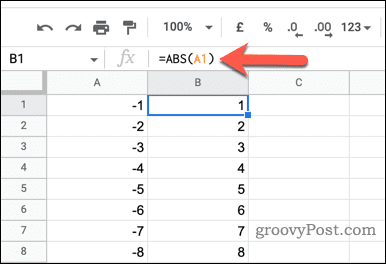
Once you have entered the ABS function in the cell, any negative values you have used will be converted to positive. For example, if you use the ABS function to find the absolute value of -5, the result will be 5.

If you use the ABS function to find the positive value of 5, the result will also be 5. This is because ABS can only return absolute values. If the value is already absolute (and thus positive), it doesn’t change it.

How to Convert Negative Numbers to Positive Using an IF Formula

The IF function allows you to perform a test. In simple terms, this is a TRUE or FALSE test. An IF formula will test if something is X. If it is, do Y, or otherwise do Z.

This function can be useful for converting negative numbers to positive numbers because it allows you to test whether a number is negative or positive. If it is negative, then IF can return the absolute value of the number, turning it into a positive. If it’s positive, it’ll return that value anyway.

To use the IF function to convert negative numbers to positive numbers in Google Sheets:

1. Open your Google Sheets spreadsheet.
2. Select the cell where you want the converted value to appear.
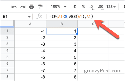
3. Type: =IF(A1<0,ABS(A1),A1) into the cell.
   • This formula tests whether the value in cell A1 is less than zero.
   • If it is, the ABS function is used to return the absolute value of the number. If it is not, the number itself is returned.
   • Replace A1 with the cell reference that contains your negative value in your spreadsheet.
4. Press Enter to apply the formula and return the result.
   

At this point, any negative values that you have used in the formula will be converted into positive values. If the value in cell A1 is negative, the absolute value will be returned. If the value is positive or zero, the value itself will be returned.

How to Convert Negative Numbers to Positive Using the SIGN Function

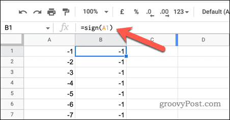
The SIGN function in Google Sheets returns 1 if a number is positive, -1 if it is negative, and 0 if it is zero. You can use the SIGN function to convert negative numbers to positive numbers in Google Sheets by using it in combination with other functions, such as multiplication or addition.

To use the SIGN function in Google Sheets:

1. Open your Google Sheets spreadsheet.
2. Select the cell where you want to convert the negative number to a positive number.
3. Type: =SIGN(number) into the cell and replace number with the cell reference or value that you want to convert.
4. Press Enter to apply the formula and see the result. The cell will now display the sign of the number that you entered, either 1 (for positive numbers), -1 (for negative numbers), or 0 (for zero).
   
5. To convert the negative number to a positive number, you’ll now need to use the SIGN function in combination with another function—in this case, a simple multiplication. For example, you can use the formula =A1*SIGN(A1) to convert the number in cell A1 to its absolute value.
   

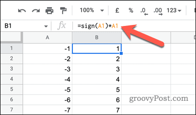
At this point, any values that you have used with the SIGN function will be converted to a positive number. You can use the SIGN function elsewhere in your spreadsheet to convert multiple negative numbers to positive numbers.

Data Analysis in Google Sheets

Using the steps above, you can quickly convert negative numbers to positives in Google Sheets. These methods can help you to better understand and analyze your data, as well as make it easier to work with formulas and perform calculations.

Want to look closely at how your spreadsheet is working? Knowing how to show formulas in Google Sheets can also be helpful, as it allows you to see the deeper methods in use behind the calculations (and troubleshoot any problems).

You can also use the search functionality in Google Sheets to quickly locate specific cells or data points. You might also find that copying values and not formulas can be useful when you want to preserve original data before you make changes to your data set.